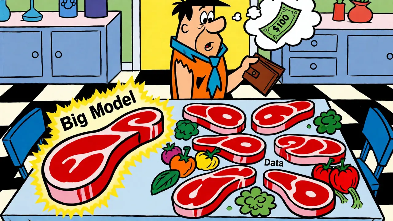
Imagine you have a fixed budget of $100 to spend on a dinner party. Do you buy one massive steak and no sides, or five medium steaks with plenty of vegetables? For years, the AI industry treated Large Language Model (LLM) training like that first option: buy the biggest model possible, even if it meant starving it of data. Then in 2022, researchers at DeepMind published a paper that flipped this logic on its head. They showed that for every parameter in your model, you need roughly 20 tokens of training data. This is known as the Chinchilla scaling law. If you ignore this ratio, you are wasting compute power. You are either building a brain too big for the information it can absorb, or a dataset too small to teach a smaller brain effectively.
This article breaks down why the Chinchilla optimal ratio matters, how to calculate it for your own projects, and where these rules start to break down. We will look at the math behind the magic, compare it to previous approaches like GPT-3, and give you a practical checklist for allocating resources in 2026.
The Core Discovery: Balanced Scaling
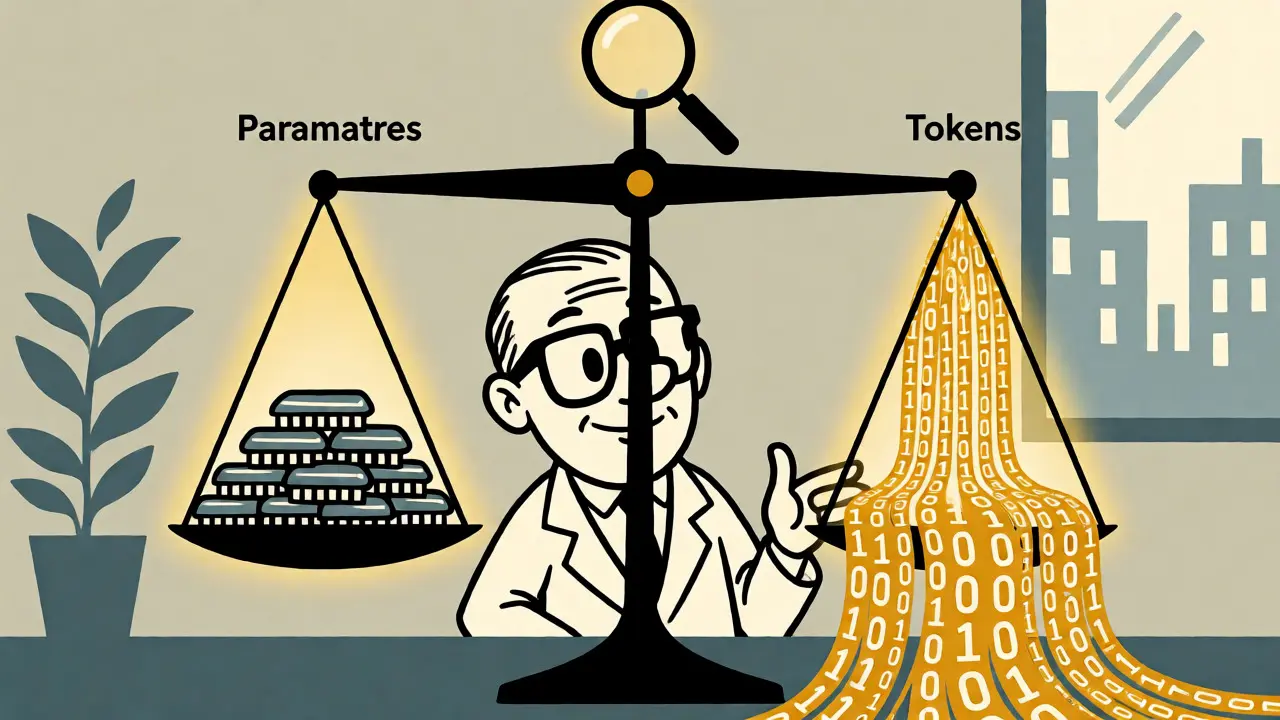
Before Chinchilla, the dominant wisdom came from Kaplan et al., who suggested that model size was more important than data volume. If you had limited compute, you should build the largest model you could afford. DeepMind’s team, led by Jordan Hoffmann and others, tested this by training over 400 transformer models ranging from 70 million to 16 billion parameters. They varied two things: the number of parameters (N) and the number of training tokens (T). They found that loss-the measure of how wrong the model is-decreases predictably when both N and T increase. But here is the kicker: they scale equally. The optimal relationship is approximately T ≈ 20N. This means if you want to train a model with 1 billion parameters, you need about 20 billion tokens. If you try to train a 10-billion-parameter model on only 50 billion tokens, you are under-training it. It has the capacity to learn more, but it never sees enough examples to fill those weights. This discovery changed the game because it proved that GPT-3, which had 175 billion parameters, was severely under-trained relative to its compute budget. It was "over-sized." To get the same performance with less compute, you could use a smaller model trained on much more data. In fact, DeepMind released their own model, Chinchilla, which had 70 billion parameters (less than half of Gopher's 280 billion) but was trained on four times more data. Chinchilla outperformed larger models on benchmarks while using significantly less energy and memory.
Why 20 Tokens Per Parameter?
You might ask, why exactly 20? Why not 10 or 50? The answer lies in the gradient signal. Each parameter in a neural network is essentially a slot for storing knowledge. During training, backpropagation updates these slots based on errors seen in the data. If you provide too few tokens per parameter, many slots remain empty or poorly optimized. The model is "under-fitted" in terms of data exposure, despite having high capacity. Conversely, if you provide way more than 20 tokens per parameter, you hit diminishing returns. The model learns what it can, and additional data doesn't improve loss significantly enough to justify the extra compute cost. The 20:1 ratio represents the sweet spot where the marginal gain in performance per unit of compute is maximized. The mathematical foundation relies on the approximation that the total floating-point operations (FLOPs) required for training is roughly $6 \times N \times T$. Here, $N$ is the number of parameters and $T$ is the number of tokens. By fixing the compute budget ($C$), we can solve for the optimal $N$ and $T$. Since $C \approx 6NT$, and we know $T \approx 20N$, we can substitute to find that $N \propto \sqrt{C}$ and $T \propto \sqrt{C}$. Both scale with the square root of your compute budget. This symmetry is what makes the scaling laws so robust across different scales.

Practical Application: Calculating Your Budget
So, how do you apply this to real-world engineering? Suppose you have a specific compute budget measured in FLOPs. Let's say you have access to a cluster that allows for $2 \times 10^{20}$ FLOPs of training. Using the Chinchilla equations, you can derive the ideal model size and dataset size. 1. Determine Total Compute: Estimate your available FLOPs. This includes hardware time multiplied by the efficiency of your training setup. 2. Solve for Parameters ($N$): Use the relationship derived from the scaling laws. For a budget of $2 \times 10^{20}$ FLOPs, the optimal model size is approximately 9 billion parameters. 3. Solve for Tokens ($T$): Multiply $N$ by 20. In this case, $9 \text{ billion} \times 20 = 180 \text{ billion tokens}$. If you stick to this plan, you maximize the performance-per-dollar of your training run. If you decide to go bigger, say 20 billion parameters, you must ensure you have 400 billion tokens ready. If you don't, you are better off shrinking the model to match your data availability. Many startups fail here: they scrape a decent amount of data, then try to squeeze it into a massive model architecture, resulting in a model that memorizes rather than generalizes.
| Strategy | Model Size Trend | Data Volume Trend | Efficiency | Example |
|---|---|---|---|---|
| Kaplan Scaling (Pre-2022) | Large increase | Moderate increase | Low (Under-trained) | GPT-3 (175B params) |
| Chinchilla Scaling (Post-2022) | Moderate increase | Large increase | High (Compute-Optimal) | Chinchilla (70B params) |
| Over-Trained Regime | Small/Medium | Very High | Diminishing Returns | Llama-3 variants |
Limits and Caveats: When 20:1 Isn't Enough
While the 20:1 ratio is a powerful heuristic, it is not a universal law of physics. It applies strictly to pretraining under a fixed compute constraint. Several factors can shift this optimal point. First, data quality matters immensely. The original Chinchilla experiments used relatively clean, diverse web text. If your dataset is noisy or highly repetitive, you might need fewer tokens per parameter because the model hits a learning ceiling faster. Conversely, if your data is extremely dense and complex (like scientific papers or code), you might benefit from more tokens per parameter to fully exploit the structure. Second, architecture changes affect the ratio. Chinchilla was based on standard Transformer architectures. Newer architectures, such as Mixture-of-Experts (MoE) models, behave differently. In MoE, only a subset of parameters is active during each forward pass. While the total parameter count is high, the effective compute per token is lower. This complicates the simple $6NT$ formula. Researchers have found that for MoE models, the optimal ratio can deviate, sometimes requiring more tokens to activate all experts effectively. Third, downstream tasks change the calculus. Chinchilla optimizes for pretraining loss. However, some downstream tasks, like reasoning or coding, may benefit from larger models even if they are slightly under-trained during pretraining. There is an ongoing debate about whether "over-training" small models (using 100+ tokens per parameter) yields better results for specific applications. Recent trends show models like Llama-3 being trained on trillions of tokens, far exceeding the 20:1 ratio. This suggests that for certain capabilities, more data is always better, provided you have the compute.
Replication and Validation
Science requires reproducibility, and Chinchilla scaling laws have held up well. Independent teams have replicated these findings. For instance, Cerebras Systems trained a series of models called Cerebras-GPT, ranging from 111 million to 13 billion parameters. They explicitly followed the 20 tokens per parameter rule and achieved state-of-the-art results for their size classes. This validation across different hardware (wafer-scale engines vs. GPU clusters) and different research groups strengthens the claim that balanced scaling is a fundamental property of neural networks, not just an artifact of DeepMind's specific setup. However, note that the exact constant varies. Some studies suggest ratios between 15:1 and 25:1 depending on the evaluation metric. The key takeaway isn't to obsess over the number 20, but to respect the principle of balance. If your model is 10x larger than the optimal size for your data, you are wasting money. If your data is 10x larger than the optimal size for your model, you are also wasting money, though perhaps less painfully since inference costs are often higher than training costs for deployed models.
Actionable Checklist for Engineers
Before you launch your next training run, run through this checklist to ensure you aren't violating basic scaling principles:
- Audit your Data-to-Parameter Ratio: Divide your total training tokens by your model parameters. Is it close to 20? If it is below 10, consider shrinking your model. If it is above 50, consider growing your model or accepting diminishing returns.
- Estimate FLOPs Accurately: Don't guess. Use the $6NT$ approximation for initial estimates, but account for attention mechanisms ($O(N^2)$ complexity) if sequence lengths are very long.
- Consider Inference Costs: A smaller, well-trained model is cheaper to serve. If you plan to deploy widely, favoring the Chinchilla optimum reduces long-term operational expenses.
- Check Data Quality: Ensure your tokens are meaningful. Padding and low-quality text inflate your token count without adding learning value, skewing your ratio calculation.
- Monitor Loss Curves: If your training loss plateaus early while you still have data left, you are likely over-trained. If loss is still dropping steeply at the end of your epoch limit, you are under-trained.
What happens if I train a large model on too little data?
You create an "under-trained" model. It has high capacity but poor generalization. It may memorize the training set (overfitting) but perform poorly on new data. Additionally, you waste computational resources on unused parameters, increasing both training and inference costs unnecessarily.
Is the 20 tokens per parameter rule still valid for modern models like Llama-3?
Modern models often exceed this ratio significantly, training on 100+ tokens per parameter. This is known as the "over-trained" regime. While Chinchilla predicts optimal efficiency at 20:1, practitioners often find that extra data improves reasoning and world-knowledge capabilities beyond what pure loss minimization predicts, especially for chat-style assistants.
How does Mixture-of-Experts (MoE) affect the Chinchilla ratio?
MoE models have many parameters but only activate a subset per token. The standard Chinchilla ratio assumes all parameters are updated per token. For MoE, the effective compute per token is lower, so the optimal data-to-active-parameter ratio remains similar, but the total parameter count can be much higher without requiring proportional increases in data.
Can I use Chinchilla laws to estimate the cost of training?
Yes. By calculating the required FLOPs ($6 \times N \times T$) for your desired model size and data volume, you can estimate the GPU-hours needed. Multiply this by the hourly rate of your cloud provider to get a baseline training cost. Remember to add overhead for checkpointing and debugging.
Does data quality change the optimal ratio?
Absolutely. Noisy or redundant data provides less unique information per token. With lower quality data, the optimal number of tokens per parameter decreases because the model saturates its learning potential sooner. High-quality, diverse data may allow or require a higher ratio to fully exploit the model's capacity.